Build a Traffic Sign Recognition Project

The goals/steps of this project are the following:

• Load the data set (see below for links to the project data set)
• Explore, summarize and visualize the data set
• Design, train and test a model architecture
• Use the model to make predictions on new images
• Analyze the softmax probabilities of the unseen photos
• Summarize the results with a written report

Data Set Summary & Exploration

1. Data Exploration

The code for this step is contained in the second code cell of the IPython notebook.

I used numpy shape attribute and the pandas library to calculate summary statistics of the traffic signs data set:

• The size of training set is 34799
• The size of test set is 12630
• The shape of a traffic sign image is 32x32x3
• The number of unique classes/labels in the data set is 43

2. Include an exploratory visualization of the dataset and identify where the code is in your code file.

The code for this step is contained in the third code cell of the IPython notebook.

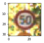
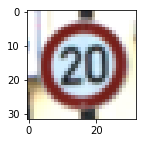
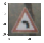
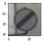
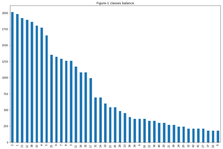
Here is an exploratory visualization of the data set. It is a bar chart showing the numbers of occurrences of each label in the data set.

Here I can see basic summary for the labels above:

• Label 2 - (“Speed limit (50km/h)”) it is the label with more example about 2000 examples
  • 
• Labels with less examples roughly between 190 - 200:
  • 0 - (“Speed limit (20km/h)”) are
    • 
  • 19 - (“Dangerous curve to the left”)
    • 
  • 32 - (“End of all speed and passing limits”)
    • 

I’ll perform some experiments in training and keep in mind that maybe data augmentation will be necessary to refining the final model.

Design and Test a Model Architecture

1. Preprocessing Data

Before starting any design or changes, I wanted to consider baseline results using the LetNet-5 Convolutional Neural Network. In the baseline step, I feed the LetNet5 with the training set and measure performance on both training and testing sets. The data feed in this step has not any pre-processing changes.

The results below shows a Baseline - Validation Accuracy = 0.878 and Baseline Test Accuracy = 0.867. With this base results, the next step is to improve them by pre-processing data and to perform design change in LetNet-5 Architecture.

*Baseline - EPOCH 1 ...
*Baseline - Validation Accuracy = 0.639
*Baseline - EPOCH 2 ...
*Baseline - Validation Accuracy = 0.755
*Baseline - EPOCH 3 ...
*Baseline - Validation Accuracy = 0.807
*Baseline - EPOCH 4 ...
*Baseline - Validation Accuracy = 0.845
*Baseline - EPOCH 5 ...
*Baseline - Validation Accuracy = 0.829
*Baseline - EPOCH 6 ...
*Baseline - Validation Accuracy = 0.837
*Baseline - EPOCH 7 ...
*Baseline - Validation Accuracy = 0.852
*Baseline - EPOCH 8 ...
*Baseline - Validation Accuracy = 0.866
*Baseline - EPOCH 9 ...
*Baseline - Validation Accuracy = 0.861
*Baseline - EPOCH 10 ...
*Baseline - Validation Accuracy = 0.878
Baseline Test Accuracy = 0.867

Preprocessed Data

The code for this step is contained in the ninth code cell of the IPython notebook.

• Normalization

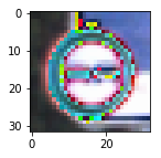
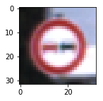
  I normalized the image data by subtracting 128 pixels from the image and then divided by 128, and it will make data be centered around zero, which it is desirable for the optimizer.

  

2. Data

The data is split into training, validation, and test sets, the sklearn function shuffle is used to randomize the training data in the fifteenth code cell of the IPython notebook.

My final training set had 90300 number of images. My validation set and test set had 4410 and 12630 number of images.

The eleventh code cell of the IPython notebook contains the code for augmenting the data set.

• Data Augmentation The training dataset was augmented with the following steps

  1. Per class randomly select an image from that class
  2. Apply randomly one of these transformations (clipped_zoom, bright_trasform, rotate_) with random parameters
  3. Append the new augmented image to a list
  4. repeat steps 1 to 3 until the number of elements of the list plus number of example of current class sums 2100
  5. append the augmented list to the current training data

  • Here is an example of an original image and an augmented Images:

  • original image

  

  • bright_trasform(8.66), clipped_zoom(0.58), rotate_(15.5)

  

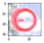
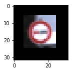
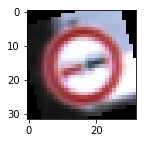
  The data augmentation only it is performed as a step in the final model to gain more accuracy.

  The difference between the original data set and the augmented data set is the following:

  • All classes have the same number of examples 2100 per class
  • The expanded dataset has 90300 images in total

3. Model Architecture

The code for my final model is located in the fourteenth cell of the Jupyter notebook.

My final model consisted of the following layers:

Layer	Description
Input	32x32x3 RGB image
Convolution 5x5x3x20	1x1 stride, ‘VALID’ padding, outputs 28x28x20
RELU
Max pooling	2x2 stride, outputs 14x114x20
Convolution 5x5x20x50	1x1 stride, ‘VALID’ padding, outputs 10x10x50
RELU
Max pooling	2x2 stride, outputs 5x5x50
Fully connected input 1250	outputs 140
RELU
DROPOUT	0.50
Fully connected input 140	outputs 100
RELU
DROPOUT	0.50
Fully connected input 100	outputs 43
Softmax

4. Training

The code for training the model is located in the fifteenth and sixteenth cells of the Jupyter notebook.

To train the model, I used an AdamOptimizer with a learning rate of 0.001, EPOCHS 15, and BATCH_SIZE 128. Two dropouts were set up to 0.75.

The model was trained inside a tensor flow session in which iterate over the EPOCHS, in each EPOCH pass training data was randomize with sklearn#shuffle function, the training operation was performed multiple times according to number of BATCHES in the training set and an accuracy measure was performed on both validation set and the last batch of the training set.

To run the training operation; the feed dictionary contains the batches for examples, labels, and the probability used for the dropout layer.

5. Experiments

The code for calculating the accuracy of the model is located in the sixteenth cell of the Ipython notebook.

• What was the first architecture that was tried and why was it chosen?

• What were some problems with the initial architecture?

• How was the architecture adjusted, and why was it changed? Typical adjustments could include selecting a different model architecture, adding or taking away layers (pooling, dropout, convolution, etc.), using an activation function or changing the activation function. One common justification for adjusting an architecture would be due to overfitting or underfitting. High accuracy on the training set but low accuracy on the validation set indicates overfitting; a low accuracy on both sets indicates underfitting.

• Which parameters were tuned? How were they adjusted and why?

• What are some of the essential design choices and why were they chosen? For example, why might a convolution layer work well with this problem? How might a dropout layer help with creating a successful model?

• What architecture was chosen?

• Why did you believe it would be relevant to the traffic sign application?

• How does the final model’s accuracy on the training, validation and test sets provide evidence that the model is working well?

I’ll try to address the questions above in next lines;

LeNet-5 was the architecture used in this project, it is a well known neural network, it appear roughly in 1998, and it is well suited to recognize visual patterns directly from pixels. LetNet-5

To achieve the results above, the first model was trained with original LeNet-5 architecture, not getting good results since both validation and test accuracies were poor, the next step was increasing the number of EPOCHS that did not help at all the validation accuracy did not overcome 0.868 and the test accuracy was 0.858 after 50 EPOCHS.

At that point, data was not normalized; the next parameter to tune was learning rate by increasing it to 0.01 both validation, and test accuracies were down to less than 0.058. Decreasing learning rate to 0.0001 with 50 epochs ends in the same result that increasing epochs for the first time. At this point, a possible conclusion is that LeNet-5 can not learn with data which is not normalized.

The next step was normalizing data and repeat training with original LetNet-5, learning rate 0.001 and 50 epochs, this time model get a Validation Accuracy = 0.945 and Test Accuracy = 0.934.

Next step was trying to add more complexity to the net by increasing filter from 6 to 20 and from 16 to 50 respectively for the two convolution layers; under the assumption that increasing filter would give to the network ability to differentiate more between 43 labels rather than ten labels. in the same sense the first two fully connected layers outputs were increase a little. Having these changes and trained with 50 epochs and rate limit of 0.001 the network training accuracy was 1.000, validation accuracy was 0.970, and test accuracy was 0.947.

Under the assumption that model it is overfitting data, two dropout layers were added to the network, the table below shows the dropouts values and its results

Dropout1	Dropout2	training accuracy	validation accuracy	test accuracy
0.75	0.75	1.0	0.953	0.931
0.50	0.75	1.0	0.966	0.956
0.50	0.50	1.0	0.978	0.965
0.30	0.50	1.0	0.972	0.956
0.50	0.30	1.0	0.969	0.966

My final model results were:

• training set accuracy of 1.000
• validation set accuracy of 0.966
• test set accuracy of 0.965

Final model parameter + data augmentation

Dropout-1	Dropout-2	training accuracy	validation accuracy	test accuracy
0.50	0.50	1.000	0.966	0.965

Despite that training accuracy and validation are kind of far from each other, and it could be an overfitting sign, the test accuracy with respect the validation accuracy looks more consistent, and they are in a right level of accuracy.

Test a Model on New Images

1. Find German traffic signs found on the web and provide them in the report.

Here are twelve German traffic signs that I found on the web:

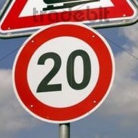
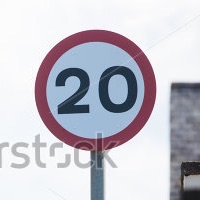
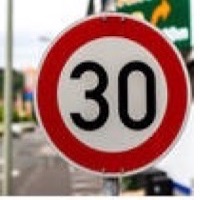
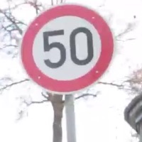
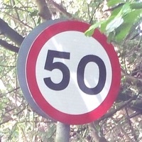
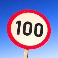
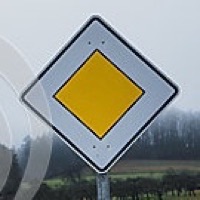
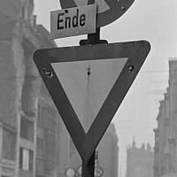
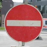
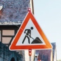
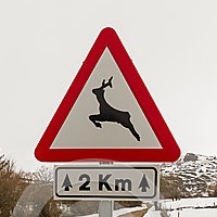
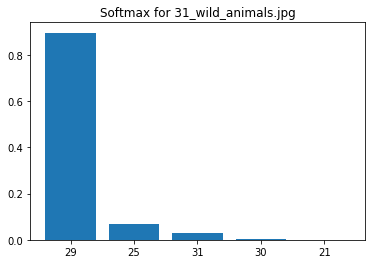
The ten images (wild animals) might be difficult to classify because it is similar to the seven (road work) or maybe the image(road work) might be classified as (wild animals)

2. Discuss the model’s predictions on new traffic signs.

The code for making predictions on my final model is located in the tenth cell of the Ipython notebook.

Here are the results of the prediction:

Image	Prediction
Speed limit (20km/h)	Speed limit (20km/h)
Speed limit (20km/h)	Speed limit (20km/h)
Priority road	Priority road
Yield	Yield
No Entry	No Entry
Speed limit (30km/h)	Speed limit (30km/h)
Road work	Road work
Speed limit (50km/h)	Keep right
Speed limit (50km/h)	Speed limit (80km/h)
Wild animals crossing	Bicycles crossing
Go straight or right	Go straight or right
Speed limit (100km/h)	Speed limit (100km/h)

The model was able to correctly guess 10 of the 12 traffic signs, which gives an accuracy of 83.33%. This compares maybe not favorably to the accuracy on the test set of 96.5%.

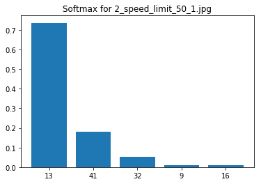
The new images are not to fit to avoid external noise provided by the behind landscape of the picture. For example, the prediction for 2_speed_limit_50_1 this image has in behind a lot of tree branches maybe that’s why the model predicted wrong this example. It should be considered to either add more example with different backgrounds or pre-process more the new data to squeeze the background and just focus the signal itself.

3. Describe model certainty

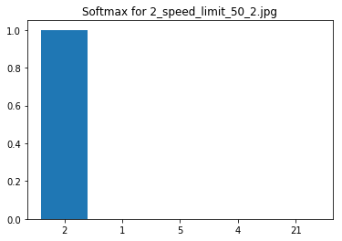
In general model it is good, there are some cases for the sign of (2-Speed limit (50km/h) -1 and (2-Speed limit (50km/h) -2 that models does not work as expected.

The code for making predictions on my final model is located in the twenty-second cell of the Ipython notebook.

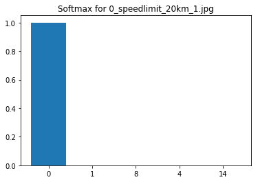
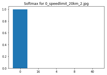
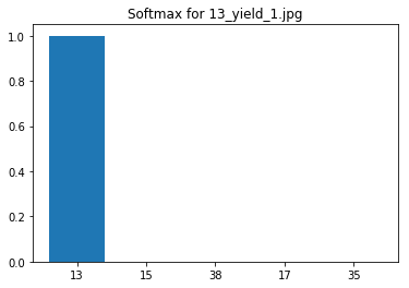
Some scores for the top 5 softmax are too small to be represented by three decimals, for that reason, there will be scores of 0.100 in one class and 0.000 in others, which means that they have tiny probabilities. But it keeps the rank.

For the 1th image:

Probability	Prediction
0.100	0-Speed limit (20km/h)
0.000	1-Speed limit (30km/h)
0.000	4-Speed limit (70km/h)
0.000	16-Vehicles over 3.5 metric tons prohibited
0.000	8-Speed limit (120km/h)

For the 2th image:

Probability	Prediction
0.999	0-Speed limit (20km/h)
0.001	16-Vehicles over 3.5 metric tons prohibited
0.000	3-Speed limit (60km/h)
0.000	8-Speed limit (120km/h)
0.000	1-Speed limit (30km/h)

For the 3th image:

Probability	Prediction
1.000	12-Priority road
0.000	0-Speed limit (20km/h)
0.000	1-Speed limit (30km/h)
0.000	2-Speed limit (50km/h)
0.000	3-Speed limit (60km/h)

For the 4th image:

Probability	Prediction
1.000	13-Yield
0.000	12-Priority road
0.000	38-Keep right
0.000	36-Go straight or right
0.000	9-No passing

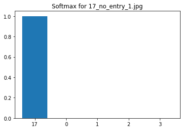
For the 5th image:

Probability	Prediction
1.000	17-No entry
0.000	14-Stop
0.000	0-Speed limit (20km/h)
0.000	1-Speed limit (30km/h)
0.000	2-Speed limit (50km/h)

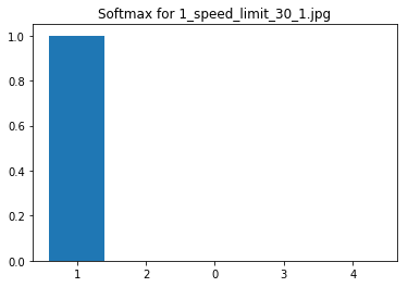
For the 6th image:

Probability	Prediction
1.000	1-Speed limit (30km/h)
0.000	2-Speed limit (50km/h)
0.000	4-Speed limit (70km/h)
0.000	6-End of speed limit (80km/h)
0.000	5-Speed limit (80km/h)

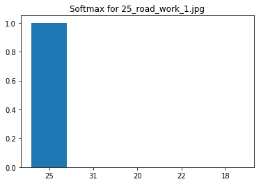
For the 7th image:

Probability	Prediction
1.000	25-Road work
0.000	31-Wild animals crossing
0.000	22-Bumpy road
0.000	20-Dangerous curve to the right
0.000	12-Priority road

For the 8th image:

Probability	Prediction
0.605	38-Keep right
0.379	13-Yield
0.010	36-Go straight or right
0.003	41-End of no passing
0.001	17-No entry

For the 9th image:

Probability	Prediction
1.000	5-Speed limit (80km/h)
0.000	7-Speed limit (100km/h)
0.000	2-Speed limit (50km/h)
0.000	3-Speed limit (60km/h)
0.000	6-End of speed limit (80km/h)

For the 10th image:

Probability	Prediction
0.897	31-Wild animals crossing
0.102	23-Slippery road
0.002	21-Double curve
0.000	29-Bicycles crossing
0.000	19-Dangerous curve to the left

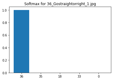
For the 11th image:

Probability	Prediction
1.000	36-Go straight or right
0.000	35-Ahead only
0.000	33-Turn right ahead
0.000	13-Yield
0.000	38-Keep right

For the 12th image:

Probability	Prediction
1.000	7-Speed limit (100km/h)
0.000	10-No passing for vehicles over 3.5 metric tons
0.000	8-Speed limit (120km/h)
0.000	5-Speed limit (80km/h)
0.000	3-Speed limit (60km/h)